I've been meaning to create a post introducing the use of the Space Analysis package for a few weeks, now, but with various trips it's been impossible to find the time. Anyway, here it is, at last.
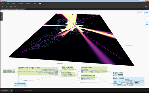
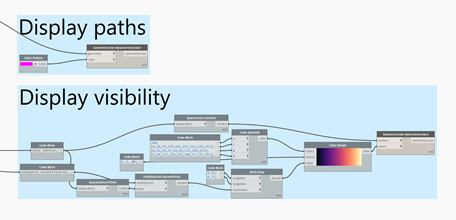
You can start by downloading the graph we'll be walking through in this post. Here's a picture of the graph, with its graphics generated.
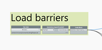
The graph is fairly simple: it loads some geometry from an SAT file that we'll use as the definition of our barriers for the SpaceLattice.
I'm using an SAT file we posted with the campus layout example that defines the buildings for the Carleton University campus. But you can easily swap this for an SAT file defined using the ACISOUT command from AutoCAD with your own geometry. The graph doesn't depend on any specific geometry being used… the intention is that you use it with 2D geometry, but it shouldn't fail if you use 3D geometry by mistake.
We then get the bounding box of this geometry – jumping through a few hoops in case it's 3D – then expand that by some distance to get dimensions of our SpaceLattice that are larger than the geometry. This is important, because if you use the bounding box of the geometry – and then use points on the bounding box as the start/end points of pathfinding, as we will do – then these points may not actually be on the lattice due to its resolution. So choosing a larger bounding box to define the lattice – or choosing points that aren't on the boundary – is a good idea.
We're going to define an axis that goes diagonally across our bounding box… we assume that the first and third corners will define a diagonal line, one way or another.
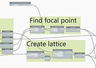
We then need to create the axis line and select a point a certain distance long it, using the slider – the main user input element to be used in the graph – to define the parameter along this diagonal axis. I've called this point the focal point – or focus – although that's not really accurate with respect to visibility (it's actually the opposite… the point from which we look around).
We also create our SpaceLattice – defined using our expanded bounding box along with the barrier geometry that we convert to line objects using a utility function for safe measure – that will be used by both pathfinding and visibility. I've chosen a resolution of 0.5, which works out to roughly 6 metres in the Carleton SAT file (it's important to check the units of the model!). For smaller indoor environments, 0.2 metres is a better choice to make sure the paths can get through small doorways. Finer resolutions come at a cost in terms of execution time, of course.
Next we use the SpaceLattice to create a PathField, using the focal point as the endpoint. (We could use another PathField creation method to specify it as the startpoint: it doesn't really matter for this graph.) A PathField allows us to calculate multiple Routes for a fixed start or endpoint with the same cost as a single Route calculation. If we only wanted a single Route, we'd just use the Route.BySpaceLattice node, passing in the start and endpoints.
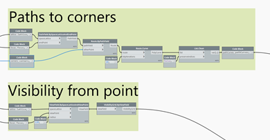
It's important to create the PathField using the focus, but then pass the corners to Route.ByPathField: if we do the other way round the graph will generate the same results, but we'll be creating four PathFields – one for each corner – rather than just one. You'll still end up with four Route objects, but you'll have missed out on the efficiencies gained by using a single PathField to find multiple Routes.
For visibility we create a ViewField – again specifying our focus as the viewPoint – with a radius that's large enough for see from one end of our bounding box to the other. In fact, rather than hardcoding this, we could also have calculated it from the length of our axis line (for instance).
Displaying the paths is simple – when all four paths are calculated, we'll see pink lines heading outwards to the four corners – but visibility is a bit more complex.
We take the Points from our SpaceLattice and use the VisibilityGrid to get the value for each one. We then use Math.Map to really only consider the range between 0.25 and 0.75: anything below 0.25 will be 0 and anything about 0.75 will be 1, with the values between 0.25 and 0.75 stretched to fit the range of 0 to 1. We do this to help compensate for some minor deficiencies in the visibility calculation algorithm that derive from it working on a grid. It helps give a more consistent blurring when "looking" at angles close to the poles, for instance.
These values then get mapped via a Color Range to the SpaceLattice's Surface.
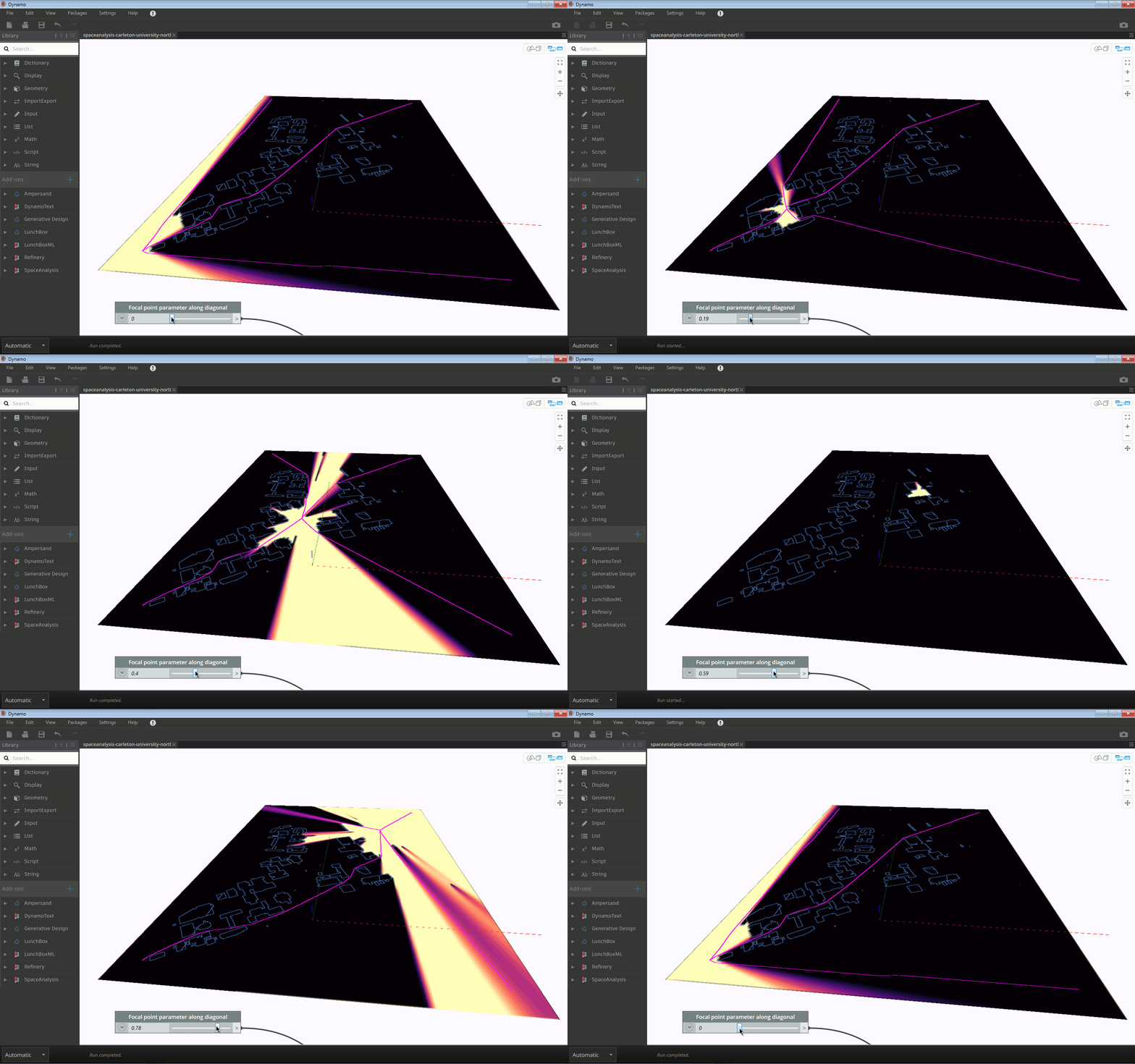
Here's an animation of the slider being adjusted from 0 to 1, to give you an idea of how it works.
Give the sample a try and let us know what you think!
This graph is really about seeing how the package works with Dynamo, of course. In a follow-up post we'll look at how we can add some metrics based on the pathfinding and visibility calculations to see what Refinery can bring to the table (al
beit with this overly simplified usage scenario).

Leave a Reply